Discrete time Markov chains

Transition probability

State transition

Recall that in a Markov process, only the last state determines the next state that the Markov process will visit:

Ҏ[ X(t+1) = x_t+1 | X(1) = x₁, X(2) = x₂, ..., X(t) = x_t ] = Ҏ[ X(t+1) = x_t+1 | X(t) = x_t ]

The state at time t is X(t)
The state at time t+1 is X(t+1)
Moving from state X(t) to the state X(t+1) is called state transition

One-step transition probability

Given that the Markov chain is in state i at time t
The probability that the Markov chain will be in state j at time t+1 is defined as:

Notice that this relationship is valid for any value of t.

I.e.:

P_ij = Ҏ[ X(t+1) = j | X(t) = i ] = Ҏ[ X(t+2) = j | X(t+1) = i ] = Ҏ[ X(t+3) = j | X(t+2) = i ]

The probability P_ij is called the one-step (state) transition probability

One-step transition probability matrix

Let N denote the number of states in the Markov chain

The collection of all one-step transition probabilities forms a matrix:

+- -+ | P₁₁ P₁₂ P₁₃ ... P_1N | | P₂₁ P₂₂ P₂₃ ... P_2N | P = | .. .. .. .. | | .. .. .. .. | | P_N1 P_N2 P_N3 ... P_NN | +- -+

Property of any one-step transition probability matrix:

P₁₁ + P₁₂ + P₁₃ + ... + P_1N = 1 P₂₁ + P₂₂ + P₂₃ + ... + P_2N = 1 .. P_N1 + P_N2 + P_N3 + ... + P_NN = 1

Stochastic matrix

Stochastic matrix

Double stochastic matrix

An N×N matrix P is a double stochastic matrix if

∀ i = 1, 2, ..., N: ∑ _{{j = 1, 2, ..., N}} P_ij = 1 and: ∀ j = 1, 2, ..., N: ∑ _{{i = 1, 2, ..., N}} P_ij = 1

(I.e., every row sum and every column sum are equal to 1)

Example Markov chain

The following Markov chain models the mode of a person:

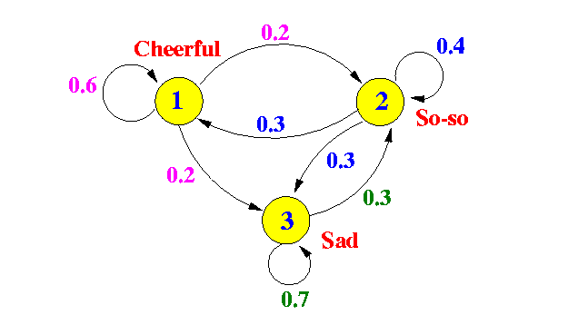
Some one-state transistion probabilities:

Ҏ[ X(t+1) = Cheerful | X(t) = Cheerful ] = P₁₁ = 0.6 Ҏ[ X(t+1) = So-so | X(t) = Cheerful ] = P₁₁ = 0.2 Ҏ[ X(t+1) = Sad | X(t) = Cheerful ] = P₁₁ = 0.2

One-step transition matrix:

+- -+ | 0.6 0.2 0.2 | P = | 0.3 0.4 0.3 | | 0.0 0.3 0.7 | +- -+

Two-steps transition probability matrix

Two steps probability:

P²_ij = Ҏ[ X(t+2) = j | X(t) = i ]

Possible ways to arrive in state j from state i in 2 steps:

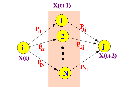
Therefore:

P²_ij = P_i1×P_1j + P_i2×P_2j + ... + P_iN×P_Nj

Note: this formula is used to multiply 2 matrices !!!

Relationship between the 2-steps and one-step transition probability matrices:

Example:

One-step transition matrix:

+- -+ | 0.6 0.2 0.2 | P = | 0.3 0.4 0.3 | | 0.0 0.3 0.7 | +- -+

Two-steps transition matrix:

+- -+ +- -+ | 0.6 0.2 0.2 | | 0.6 0.2 0.2 | P² = | 0.3 0.4 0.3 | × | 0.3 0.4 0.3 | | 0.0 0.3 0.7 | | 0.0 0.3 0.7 | +- -+ +- -+ +- -+ | 0.42 0.26 0.32 | = | 0.30 0.31 0.39 | | 0.09 0.33 0.58 | +- -+

N-steps transition probability matrix

The 2-steps transition matrix can be generalized to an N-steps process

It is easy to show that the N-steps transition matrix P^N is equal to:

P^N = P × P × ... × P

Example:

> P := matrix(3,3, [0.6, 0.2, 0.2, 0.3, 0.4, 0.3, 0.0, 0.3, 0.7]); P > evalm(P); [0.6 0.2 0.2] [ ] [0.3 0.4 0.3] [ ] [0. 0.3 0.7] P² > evalm(P&*P); [0.42 0.26 0.32] [ ] [0.30 0.31 0.39] [ ] [0.09 0.33 0.58] P³ > evalm(P&*P&*P); [0.330 0.284 0.386] [ ] [0.273 0.301 0.426] [ ] [0.153 0.324 0.523] P⁶ > evalm(P&*P&*P&*P&*P&*P); [0.245490 0.304268 0.450242] [ ] [0.237441 0.306157 0.456402] [ ] [0.218961 0.310428 0.470611] P¹⁰ > evalm(P&*P&*P&*P&*P&*P&*P&*P&*P&*P&*P); [0.2313863532 0.3075488830 0.4610647637] [ ] [0.2310495033 0.3076271722 0.4613233244] [ ] [0.2302738212 0.3078074437 0.4619187352] P²⁰ > evalm(P&*P&*P&*P&*P&*P&*P&*P&*P&*P&*P&*P&*P&*P&*P&*P&*P&*P&*P&*P); [0.2307712768 0.3076918322 0.4615368910] [ ] [0.2307701600 0.3076920917 0.4615377482] [ ] [0.2307675883 0.3076926893 0.4615397223]

It converges !!!

Initial state

Initial state π⁽⁰⁾:

Define:

π⁽⁰⁾ = ( π₁⁽⁰⁾, π₂⁽⁰⁾, ..., π_N⁽⁰⁾ )

The initial state π⁽⁰⁾ is the vector of probability values that the Markov chain is in state i with probability π_i⁽⁰⁾

Example:

Progress of a Markov chain

Starting in the initial state, a Markov process (chain) will make a state transition at each time unit.
The follow figure shows the possible ways to reach the state 1 after one step:
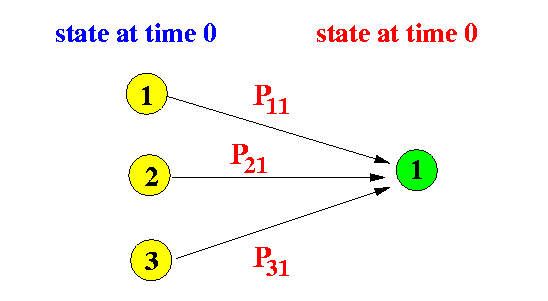
Therefore, the probability that the Markov chain is in state 1 is equal to:

The state probability vector π⁽¹⁾ = ( π₁⁽¹⁾, π₂⁽¹⁾, ..., π_N⁽¹⁾ ) after one step transition can be computed using π⁽⁰⁾ as follows:

π₁⁽¹⁾ = π₁⁽⁰⁾P₁₁ + π₂⁽⁰⁾P₂₁ + π₃⁽⁰⁾P₃₁ π₂⁽¹⁾ = π₁⁽⁰⁾P₁₂ + π₂⁽⁰⁾P₂₂ + π₃⁽⁰⁾P₃₂ π₃⁽¹⁾ = π₁⁽⁰⁾P₁₃ + π₂⁽⁰⁾P₂₃ + π₃⁽⁰⁾P₃₃
Or in matrix form: π⁽¹⁾ = π⁽⁰⁾ × P

Notice: this is a vector-matrix multiplication (rather than a matrix-vector multiplication)

Multiple steps:

2 steps: π₁⁽²⁾ = π₁⁽¹⁾P₁₁ + π₂⁽¹⁾P₂₁ + π₃⁽¹⁾P₃₁ π₂⁽²⁾ = π₁⁽¹⁾P₁₂ + π₂⁽¹⁾P₂₂ + π₃⁽¹⁾P₃₂ π₃⁽²⁾ = π₁⁽¹⁾P₁₃ + π₂⁽¹⁾P₂₃ + π₃⁽¹⁾P₃₃ Or: π⁽²⁾ = π⁽¹⁾ × P = (π⁽⁰⁾ × P) × P = π⁽⁰⁾ × (P × P) = π⁽⁰⁾ × P²
In general: π^(k) = π⁽⁰⁾ × P^k

Example:

(Maple) > x := vector([1,0,0]); > x = matrix(3,1, [1,0,0]); > P := matrix(3,3, [0.6, 0.2, 0.2, 0.3, 0.4, 0.3, 0.0, 0.3, 0.7]); x⁽¹⁾ > evalm( x&*P ); [0.6, 0.2, 0.2] x⁽²⁾ > evalm( x&*P&*P ); [0.42, 0.26, 0.32] x⁽⁴⁾ > evalm( x&*P&*P*P&*P ); [0.2832, 0.2954, 0.4214] x⁽⁸⁾ > evalm( x&*P&*P*P&*P&*P&*P*P&*P); [0.23490798, 0.30673034, 0.45836168] x⁽¹⁶⁾ > evalm( x&*P&*P*P&*P&*P&*P*P&*P&*P&*P*P&*P&*P&*P*P&*P); [0.2307951062, 0.3076862941, 0.4615185997] x⁽²⁴⁾ > evalm( x&*P&*P*P&*P&*P&*P*P&*P&*P&*P*P&*P&*P&*P*P&*P&*P&*P*P&*P&*P&*P*P&*P); [0.2307693926, 0.3076922701, 0.4615383374]

It converges !!!

Stationary state
- The stationary state is the following limiting probability:
  The stationary state is also called the steady state

Transient state: introduced through an example of Markov chain

Consider the following Markov chain:

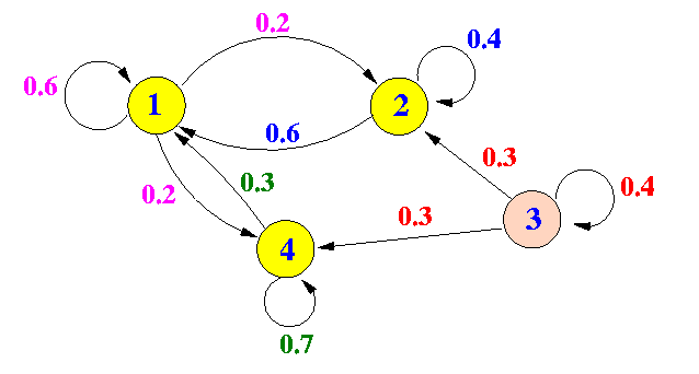
The multi-step probability matrices:

> P := matrix(4,4, [0.6, 0.2, 0.0, 0.2, \ 0.6, 0.4, 0.0, 0.0, \ 0.0, 0.3, 0.4, 0.3, \ 0.3, 0.0, 0.0, 0.7] ); P² > evalm( P&*P ); [0.54 0.20 0. 0.26] [ ] [0.60 0.28 0. 0.12] [ ] [0.27 0.24 0.16 0.33] [ ] [0.39 0.06 0. 0.55] P⁴ > evalm( P&*P&*P&*P ); [0.5130 0.1796 0. 0.3074] [ ] [0.5388 0.2056 0. 0.2556] [ ] [0.4617 0.1794 0.0256 0.3333] [ ] [0.4611 0.1278 0. 0.4111] P⁴ > evalm( P&*P&*P&*P*P&*P*P&*P ); [0.50167962 0.16834628 0. 0.32997410] [ ] [0.50503884 0.17170552 0. 0.32325564] [ ] [0.49901697 0.16699434 0.00065536 0.33333333] [ ] [0.49496115 0.16162782 0. 0.34341103] P¹⁶ > evalm( P&*P&*P&*P*P&*P*P&*P&*P&*P&*P*P&*P*P&*P&*P ); [0.5000282111 0.1666948777 0. 0.3332769112] [ ] [0.5000846332 0.1667513000 0. 0.3331640668] [ ] [ -6 ] [0.4999993559 0.1666668815 0.4294967296 10 0.3333333333] [ ] [0.4999153666 0.1665820333 0. 0.3335025999]

Note:

The probability that the Markov chain is found in state 3 becomes smaller and smaller with time !!!

Miscellaneous definitions

Transient state:
Recurrent state:
Example:
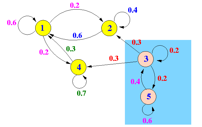
States 3 and 5 are transient states because once the Markov chain leaves theses states, it will never return back to them.

Periodic states:

A periodic state is a special subclass of recurrent states
A recurrent state i is periodic with a period d if:
I.e., a periodic state with a period d will re-occur after exactly d steps

Example:

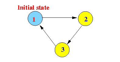
The period of the above Markov process is 3:

p⁽¹⁾11 = 0 (from state 1, in one step, we reach state 2) p⁽²⁾11 = 0 (from state 1, in one steps, we reach state 3) p⁽³⁾11 = 1 (from state 1, in one steps, we reach state 1)

Reachable state:

A state j is reachable from a state i iff:
I.e., there is a non-zero probability that we end up in state j starting from state i after a finite number of steps n

Example:

State 1 is reachable from state 3
State 3 is not reachable from state 1

Communicating states:
Example:

Chain:

A chain C is a set of states where all members are mutually communicating

I.e.:

∀ i, j ∈ C: i is reachable from j and j is reachable from i

Single chain Markov process:
Example:

State-state property of Single Chain Markov processes

The steady state probability (limiting state probability) of a state is the likelihood that the Markov chain is in that state after a long period of time
Mathematically speaking: we must find this limit

Lemma 1:

If a Markov Chain has a single chain and no periodic states, then: the limiting state probabilities exists and independent from the initial state
I.e.:
independent from the value of π⁽⁰⁾_j

No proof; but you have seen a few examples above....

Computing steady-state probabilities (limiting state probabilities)

Example Markov chain:

One-step probability matrix:

+- -+ | 0.6 0.2 0.2 | P = | 0.3 0.4 0.3 | | 0.0 0.3 0.7 | +- -+

The example Markov chain has:
According to Lemma 1, the Markov chain has a steady state and the steady state is reached from any initial state
See: click here

Finding the steady-state probability π

When Markov chain starts in initial state π⁽⁰⁾ and make 1 step:

π₁⁽¹⁾ = π₁⁽⁰⁾P₁₁ + π₂⁽⁰⁾P₂₁ + π₃⁽⁰⁾P₃₁ π₂⁽¹⁾ = π₁⁽⁰⁾P₁₂ + π₂⁽⁰⁾P₂₂ + π₃⁽⁰⁾P₃₂ π₃⁽¹⁾ = π₁⁽⁰⁾P₁₃ + π₂⁽⁰⁾P₂₃ + π₃⁽⁰⁾P₃₃ Or: π⁽¹⁾ = π⁽⁰⁾ × P

If the Markov chain is in the steady state, and makes one step, the next state equal to the steady state.
Therefore, in the steady state π = (π₁, π₂, π₃), we have:
These equations will allow you to solve for π = (π₁, π₂, π₃)

Caveat in solving for π

The system of equations obtained from the one step transition probability matrix is a dependent system of equations because one of the equation is a linear combination of the other two equations:

π₁ = π₁P₁₁ + π₂P₂₁ + π₃P₃₁ π₂ = π₁P₁₂ + π₂P₂₂ + π₃P₃₂ + π₃ = π₁P₁₃ + π₂P₂₃ + π₃P₃₃ --------------------------------------- π₁ + π₂ + π₃ = π₁(P₁₁ + P₁₂ + P₁₃) + π₂(P₂₁ + P₂₂ + P₂₃) + π₃(P₃₁ + P₃₂ + P₃₃) Facts: P₁₁ + P₁₂ + P₁₃ = 1 P₂₁ + P₂₂ + P₂₃ = 1 P₃₁ + P₃₂ + P₃₃ = 1
=> π₁ + π₂ + π₃ = π₁ + π₂ + π₃

In order to obtain a non-dependent system of equations, you must replace any one equation in the system of equations with this equation:
and then solve it.

Example:

Steady state probability satisfies:

π₁ = 0.6 π₁ + 0.3 π₂ + 0.0 π₃ .... (1) π₂ = 0.2 π₁ + 0.4 π₂ + 0.3 π₃ .... (2) π₃ = 0.2 π₁ + 0.3 π₂ + 0.7 π₃ .... (3)
And: π₁ + π₂ + π₂ = 1 .... (4)

Drop equation (3) and re-write into canonical form:

-0.4 π₁ + 0.3 π₂ + 0.0 π₃ = 0 .... (1) 0.2 π₁ - 0.6 π₂ + 0.3 π₃ = 0 .... (2) π₁ + π₂ + π₃ = 1 .... (4)

Solution using Maple:

> eq1 := -0.4*x1 + 0.3*x2 + 0.0*x3 = 0; eq1 := -0.4 x1 + 0.3 x2 = 0 > eq2 := 0.2*x1 - 0.6*x2 + 0.3*x3 = 0; eq2 := 0.2 x1 - 0.6 x2 + 0.3 x3 = 0 > eq3:= x1 + x2 + x3 = 1; eq3 := x1 + x2 + x3 = 1
> solve( {eq1, eq2, eq3}, {x1, x2, x3} ); {x1 = 0.2307692308, x2 = 0.3076923077, x3 = 0.4615384615}

Better:

> eq1 := -4/10*x1 + 3/10*x2 = 0; 2 x1 3 x2 eq1 := - ---- + ---- = 0 5 10 > eq2 := 2/10*x1 - 6/10*x2 + 3/10*x3 = 0; x1 3 x2 3 x3 eq2 := ---- - ---- + ---- = 0 5 5 10 > eq3:= x1 + x2 + x3 = 1; eq3 := x1 + x2 + x3 = 1
> solve( {eq1, eq2, eq3}, {x1, x2, x3} ); {x1 = 3/13, x2 = 4/13, x3 = 6/13}

A common way to find equilibrium equations for Markov chains

Consider the Markov transition diagram:
Focussing only on the possible ways to get to the state 1, we see:
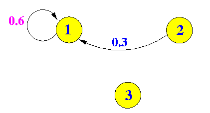
This give rise to the following equilibrium equation:
Focussing only on the possible ways to get to the state 2, we see:
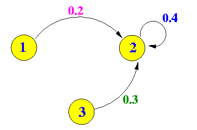
This give rise to the following equilibrium equation:
Focussing only on the possible ways to get to the state 3, we see:
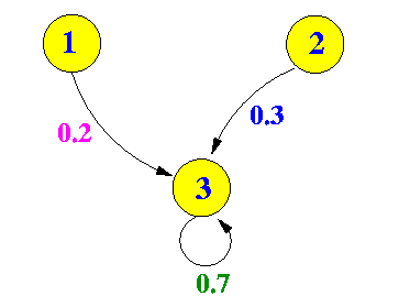
This give rise to the following equilibrium equation:

Note:

In more complicated Markov chains, we may need to use multiple transitions to establish equilibrium equations
When multiple transitions are used, we treat it like a multi-step transition (See: click here )