---

Queues and the Poison arrival process to queues

---

• Queueing System
  • A queueing system consists of:

    An arrival process of client into a holding area (queue) Clients come (enter in) to the queueing system to obtain a certain service A queue management process that organizes the clients in the queue The most commonly used queue management processes: FIFO A service process that fullfills the service requests of clients After obtaining the service from the server, a client will leave the queueing system We call this process the departure process

    Schematically:

  ---

  ---

• Interesting measures of a queueing system
  • Interesting (relevant) performance measures:

    Average waiting time inside the queue I.e., what is the average time that customers must wait before they starts obtaining the service Average time spent in system I.e., what is the average time needed for customers to complete the service (This is the duration from the arrival of the customer to its departure)

  ---

  ---

  Review of Probability Theory

  ---

  ---

• Probability mass/density function and Probability distribution function
  • The probability distribution function a discrete random variable is known as a probability mass function.

    The probability distribution function a continuous random variable is known as a probability density function.

    ---

  • The probability mass/density function is:

    A mathematical function used to model the frequencies (probabilities) of occurrences of each event          Specifically: p(k) = Probab[ x = k ] p(k) is the probability that the outcome is equal to k (x is called a random variable)

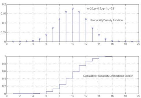
    Example: the probability mass/density function for Binomial(p, n) is:

    p(k) = C(n, k) pk (1 - p)n-k n! = ---------- pk (1 - p)n-k k!(n-k)!

    ---

    ---

  • The (cumulative) probability distribution function is the cumulative sum of the values of the probability density function:

    Discrete p(x): Q(k) = Ҏ[ x ≤ k ] = &sum x ≤ k p(x) Continuous p(x): Q(k) = Ҏ[ x ≤ k ] = &int x ≤ k p(x) Note that: d Q(x) p(x) = ------ dx

    Property of every probability distribution function:

    lim (x → ∞) Q(x) = 1

    ---

    ---

  • Example: Binomial(0.5, 20)

  ---

  ---

  ---

  ---

• Stochasitic process
  • Deterministic process:

    A deterministic process is a process with a determined schedule of events We can tell what event will happen next.

    Example: sorting algorithm

    ---

  • Stochastic process:

    A stochastic process is a process with a probabilistic schedule of events The next event will occur with a certain probability

    Example: post office (when the next cunstomer arrive is a probabilitic event)

  ---

  ---

• Poisson process
  • The Poisson process is a stochastic event where:

    1. Ҏ[ one customer arrives in the next time interval Δt ] = &lambda×t + o(Δt) ........ (1) 2. Ҏ[ no customer arrives in the next time interval Δt ] = 1 - &lambda×t + o(Δt) ........ (2) 3. Ҏ[ ≥ 2 customers arrive in the next time interval Δt ] = o(Δt) ........ (3) 4. The arrivals in non-overlapping time intervals are (probabilistically) independent

    Note:

    The notation Ҏ[x] means the probability of the event x The parameter λ is the arrival rate I.e., λ = average number of arrivals per time unit Equation (1): Ҏ[ one customer arrives in the next time interval Δt ] = &lambda×t + o(Δt) states that the probability of an arrival in the Poisson process is linearly dependent on the arrival rate λ The notation o(Δt) means: o(Δt) lim Δt &rarr 0 ------- = 0 Δt I.e., terms of the order o(Δt) are negligible compared to the term Δt

  ---

  ---

• The probabibility density function of the Poisson arrival process
  • The probabibility density function of the Poisson arrival process with arrival rate &lambda is defined as:

    p(k) = Ҏ( k arrivals in an interval T )

    Graphically:

    k arrival events | | | | V V V V |<--------------------->| T sec

    ---

  • Computing p(k)

    Divide the interval into n pieces: ΔT = T/n <--> |<-->|<-->|<-->|................|<-->| <----------------------------------> T sec By Equation (1) (click here), the probability that one customer arrives in the interval ΔT is: Ҏ[ 1 arrival in ΔT ] = λ × ΔT + o(ΔT) ~= λ × ΔT = λ × T/n The probability that k customers arrives in the interval T is a Binomial trial with probability of success equal to λ × ΔT + o(ΔT) Therefore: n! Ҏ[ k arrivals in T ] = ----------- (Ҏ[ 1 arrival in ΔT ])k (1 - Ҏ[ 1 arrival in ΔT ])n-k k! (n-k)! n! = lim (n → ∞) ----------- (λ × ΔT)k (1 - λ × ΔT)n-k k! (n-k)! Sub: ΔT = T/n n! = lim (n → ∞) ----------- (λT/n)k (1 - λT/n)n-k k! (n-k)! n! = lim (n → ∞) ----------- (λT)k × (1/n)k × (1 - λT/n)n-k k! (n-k)! Move terms that are independent of n out of the limit... (λT)k n! = -------- × lim (n → ∞) -------- (1/n)n × (1 - λT/n)n-k k! (n-k)! (λT)k = -------- × lim (n → ∞) n (n-1) ... (n-k+1) (1/n)k × (1 - λT/n)n-k k! (λT)k n (n-1) ... (n-k+1) = -------- × lim (n → ∞) ------------------- × (1 - λT/n)n-k k! n n ... n n - x ------- → 1 when n &rarr ∞ for any constant x n lim (n → ∞) (1 - λT/n)n-k = lim (n → ∞) (1 - λT/n)n × lim (n → ∞) (1 - λT/n)-k = lim (n → ∞) (1 - λT/n)n × (1 - 0)-k = lim (n → ∞) (1 - λT/n)n = e-λT (a well-known Math limit) Hence: (λT)k Ҏ[ k arrivals in T ] = ------- e-λT ........ (Poisson distribution) k!

  ---

  ---

  ---

  ---

• Expected value or the mean (average) number of a random variable
  • Definition: expected value

    The expected value of a random variable is the mean/average value of the random variable

  • Mathematical definition of expected value:

    x is a random variable with a density function Ҏ[x] (Ҏ[x] is a short hand for Ҏ[x = x]) The expected value E[x] of x is: E[x] = ∑ (all values k) k Ҏ[k]

  ---

  ---

• Expected value or the mean (average) number of a Poisson λ distributed random variable
  • By the definition of expected value:

    E[x] = ∑ (all values k) k Ҏ[k] (λT)k = ∑ (k = 0 .. ∞) k × ------ e-λT k! (λT)k = ∑ (k = 1 .. ∞) ------ e-λT (k-1)! Move terms independent of k out of the sum.... (λT)k E[x] = e-λT × ∑ (k = 1 .. ∞) ----------- (k-1)! Adjust the running index (make k run from 0 &rarr ∞).... (λT)k+1 E[x] = e-λT × ∑ (k = 0 .. ∞) ------- k! Move one term λT out of the sum... (λT)k E[x] = λT × e-λT × ∑ (k = 0 .. ∞) ------- k! Well-known Math serie: ∑ (k = 0 .. ∞) xk/k! = ex E[x] = λT × e-λT × eλT = λT

  ---

  ---

• Arrival rate of a Poisson arrival process
  • Previously, we found that the expected value of a Poisson λ distributed random variable x is:

    E[x] = λT

    The random variable x represents the number of arrivals in a time interval of duration T (See: click here )

    ---

  • Therefore:

    The average (mean) number of arrivals over a time interval of duration T is equal to λ × T

    In other words:

    The average number of arrivals per time unit is: Avg # arrivals per second = λT/T = λ

    ---

  • Arrival rate of a Poisson process

    λ is the arrival rate of the Poisson arrival process λ = the average number of arrivals per time unit (sec)

  ---

  ---

  ---

  ---

• Distribution of the interarrival times: time between 2 consecutive arrivals
  • Define:

    y = the random variable representing the time between 2 consecutive arrivals in a Poisson arrival process ( y = the inter-arrival time)

    ---

  • Probability density function of y:

    Ҏ[ y > t ] = Ҏ[ no arrivals in interval (0..t) ] (λt)0 = ----- e-λt 0! = e-λt Ҏ[ y ≤ t ] = 1 - Ҏ[ y > t ] = 1 - e-λt .... (Probability distrubution function of y)

    ---

    ---

  • Probability density function of y:

    d Q(t) p(t) = ------ ..... (from Probability theory) dt Qy(t) = 1 - e-λt Therefore: d [1 - e-λt] py(t) = ------------ dt = - e-λt × (-λ) = λ e-λt .....(Probability density function of y)

  ---

  ---

  ---

  ---

• Memory-less property of the Poisson arrival process
  • Memoryless property:

    A process is memory-less if it has the following property: Ҏ[ no event time within next t sec | event has not happened for u sec ] = Ҏ[ no event time within next t sec ] In other words: The likelihood (probability) of when the next event will happen will next be affected by the given knowledge that the event has not happened for some time

    ---

  • Example of memory-full processes:

    Volcano eruptions: The probability that a volcano will not erupt within the next 100 yrs is greatly decreased if we knew that the volcano has not erupted for 1 million years Hunger: The probability that a person does not become hungry within the next hour is greatly decreased if we knew that the person has not eaten for 6 hours

    ---

    ---

  • Memory-less property of the Poisson arrival process:

    Ҏ[ no arrival occurs within next t sec | no arrival for u sec ] = Ҏ[ no arrival occurs within next t sec ]

    Proof:

    Ҏ[ no arrival occurs within next t sec | no arrival for u sec ] = Ҏ[ no arrival occurs within next t sec and no arrival for u sec ] = ------------------------------------------------------------------ (def of cond probability) Ҏ[ no arrival for u sec ] Observe that: |<------ u ------>|<--------- t ------> ------+------------------+---------------------> 0 arrivals 0 arrival Ҏ[ no arrival occurs within next t sec and no arrival for u sec ] = Ҏ[ no arrival occurs within next t+u sec ] Therefore: Ҏ[ no arrival occurs within next t sec | no arrival for u sec ] = Ҏ[ no arrival occurs within next t+u sec ] = ------------------------------------------------ Ҏ[ no arrival occurs within next u sec ] (λ(t+u))0 --------- e-λ(t+u) 0! = -------------------- (λt)0 ----- e-λu 0! e-λ(t+u) = -------- e-λu = e-λt Also: (λt)0 Ҏ[ next arrival occurs within next t sec ] = ------ e-λt 0! = e-λt Hence: Ҏ[ no arrival occurs within next t sec | no arrival for u sec ] = Ҏ[ next arrival occurs within next t sec ] for the Poisson arrival process